Relational Database Design and Implementation
Published:
Introduction
During my dissertation research, I compiled a database encompassing dissolved CO2 estimates from flowing freshwaters across the United States spanning the years 1990 to 2020 (CDFLOW). In addition to the original database, I augmented it with supplementary data sourced from various entities, including the United States Geological Survey (USGS), Environmental Protection Agency (EPA), and numerous other government agencies focused on natural resources. In line with my forward-looking perspective as a data scientist, I endeavored to enhance the impact of my academic work by aligning the treatment of my dissertation data with industry standards. This undertaking involves the migration and structuring of academic data into a PostgreSQL relational database, emphasizing a professional data science methodology. The primary goal is not only to showcase the depth of my dissertation findings but also to underscore the practical relevance of my skills.
Within this project I will go through the creation, design, and implementation of my DB, which I will refer to as CDFLOW-EXT (Note: when I refer to just CDFLOW I am referring to the original published DB). Finally, I will demonstrate the power of the relational DB through two use cases.
Database Creation
As stated, the relational database (DB) is housed under a PostgreSQL system. However, to interface with the relational DB I used DBeaver, a free cross-platform DB tool. I think the pairing of these two open-source and free programs provide a powerful framework for working with relational DBs.
Adding Tables
I’ll skip how I setup the aforementioned software’s, there are tons of great resources to get people up and running with them.
Once, I had a Postgres server running on my local machine I created a connection with DBeaver. Within DBeaver, I created a new DB called “CDFLOW-EXT”. Now with my DB created I was able to start adding tables. To actually add the tables I imported the data via an R-script. I used R because all the data analysis for my dissertation research was completed in R and the data was already housed in an R-project saved as .RDS files. This actually points to another benefit of Postgres, which is that pretty much all programming languages can interface to edit and query Postgres DBs.
To add a table to a DB using an R-script I had to load the data in, establish a connection with the DB, write the table, then end the connection. Below is a snippet of code of what that looked like for the first table which includes the original published CDFLOW data.
# Load the data
CDFLOW <- read_csv("CDFLOW.csv")

# Establish a connection the the DB
con <- DBI::dbConnect(RPostgres::Postgres(),
               dbname = "CDFLOW-EXT",
               port = "5432")

# Write the table
dbWriteTable(con, 'CDFLOW-EXT', CDFLOW, row.names=FALSE)

# Disconnect from DB
dbDisconnect(con)
There was a total of 10 tables in the relational DB at the time of writing this (my dissertation is not complete thus more data may be added). I won’t go through the code of adding each individual table because it’ll be repetitive and looks the same as the code above. However, I will expand on the additional tables below.
Each table adds to the original table in some way to aid in data visualization or the statistical analysis of the original CDFLOW dataset. If your curious about the analysis, you’ll have to read my dissertation once it’s complete. For each of the tables I have created a table below which lists the table, what’s included in it, and how it is connected to the original data. When tables have two or more connections, they are indicated by arrows like in the case of HUC2 TABLE that means that the connections to CDFLOW is through two or more tables. Continuing with HUCTABLE as an example it connects to Site_Lookup first *via HUC12, then to CDFLOW _via* MonitoringLocationIdentifier.
| Table Name | Description of Data | Connection to CDFLOW | Original format |
|---|---|---|---|
| CDFLOW | estimates of CO2 | Original Data | .csv |
| Site_Lookup | Connection to various spatial resoultions | MonitoringLocationIdentifier | .csv |
| HUC_Table | All Nested HUCs (HUC12-HUC2) | Site_Lookup (HUC12) -> MonitoringLocationIdentifier | .csv |
| HUC2_Geo | HUC2 spatial data | HUC_Table (HUC2) -> Site_Lookup (HUC12) -> MonitoringLocationIdentifier | .shp |
| HUC8_Geo | HUC8 spatial data | HUC_Table (HUC8) -> Site_Lookup (HUC12) -> MonitoringLocationIdentifier | .shp |
| HUC8_WSIO | HUC8 Environmental data | HUC_Table (HUC8) -> Site_Lookup (HUC12) -> MonitoringLocationIdentifier | .xlsx |
| COMID_Landcover | Landcover classifications by COMID | Site_Lookup (COMID) -> COMID | .csv |
| COMID_NHD | National Hydrological Dataset COMID data | Site_Lookup (COMID) -> COMID | .shp |
| COMID_NLDI | Network Linked Data Index by COMID | Site_Lookup (COMID) -> COMID | .csv |
| State_Geo | State Spatial data | State | .shp |
With all the tables added to the CDFLOW-EXT Postgres DB I formally made the connections with some SQL. For each table I first identified the Primary key, which is the unique value for each row in the table. Then, foreign keys could be added to the tables to make the connections as indicated in the above table. If you are not familiar, a foreign key for one table must be the primary key the table you are connecting it to.
For instance, below I have included some example SQL code of how I created Primary and Foreign keys for the original CDFLOW table.
Making connections
-- First, assign the primary key for CDFLOW.
ALTER TABLE public."CDFLOW"
ADD CONSTRAINT cdflow_pk
PRIMARY KEY ("Obs_Id")

-- Next, assign the primary key in another table
ALTER TABLE public."Site_Lookup"
ADD CONSTRAINT site_lookup_pk
PRIMARY KEY ("MonitoringLocationIdentifier")

-- Then the primary key can be set as the foreign key in the OG table
ALTER TABLE public."CDFLOW"
ADD CONSTRAINT cdflow_site_lookup_fk
FOREIGN KEY ("MonitoringLocationIdentifier")
REFERENCES "Site_Lookup"("MonitoringLocationIdentifier")
Similar SQL code as the snippet above was run for each of the connections indicated in the table of tables. Now, I understand that the connections and keys might be a little confusing so a great way to visualize the relational database is through an Entity Relationship (ER) Diagram. The great news is that DBeaver automatically generates one based on the setup of a relational DB.
ER Diagram
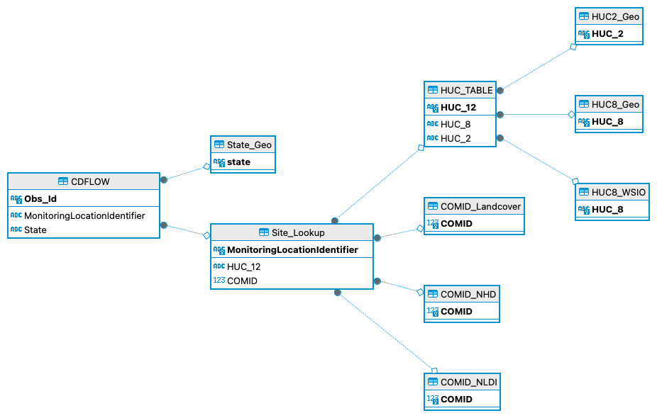
Above you will find an ER Diagram which shows the relational DB and how all the tables are related. I know there are some different ways I could have designed the DB but I find this one to be the easiest for me to work with.
Database Use Cases
Now that I have displayed the creation and deign of this database, I would like to show how I have implemented it into my workflow through two use cases. I will avoid getting in the weeds about the science behind this DB (you can read my dissertation for that). The use cases include a short modeling exercise and the creation on an interactive data visualization with Tableau.
Modeling
Now, for the sake of brevity and staying out of the weeds of my research let’s say I am interested in the percent of land classified in a watershed surrounding a flowing freshwater section. Specifically, I am interest in modeling how urban landcover might affect the average pCO2 in flowing freshwaters across HUC8s in the US. HUCs as watershed designations and follow a nested system of classification. HUC8s are a common spatial level to analyze ecological data. Again, the details are not important here. I only want to display the relational DB in action.
First, I will write an SQL sript in DBeaver to gather the correct data.
-- Query percent urban by HUC8, the left join to average CO2 by huc8 where data is not missing
SELECT "% Urban in WS (2016)" as urban, ave."HUC_8", ave.mean
FROM public."HUC8_WSIO" hw
left join
	(SELECT avg("pCO2.uatm") AS mean, ht."HUC_8" FROM public."CDFLOW" cd
	left join public."HUC_TABLE" ht
	on cd."HUC_12" = ht."HUC_12"
	Group By "HUC_8") ave
on hw."HUC_8" = ave."HUC_8"
where mean is not null
The preceding SQL code worked as intended so now I need to write this query in an R environment.
con <- DBI::dbConnect(RPostgres::Postgres(),
                      dbname = "CDFLOW",
                      port = "5432")

mod_df <- RPostgres::dbGetQuery(con, statement = '
        SELECT "% Urban in WS (2016)" as urban, ave."HUC_8", ave.mean
        FROM public."HUC8_WSIO" hw
        left join
        	(SELECT avg("pCO2.uatm") AS mean, ht."HUC_8" FROM public."CDFLOW" cd
        	left join public."HUC_TABLE" ht
        	on cd."HUC_12" = ht."HUC_12"
        	Group By "HUC_8") ave
        on hw."HUC_8" = ave."HUC_8"
        where mean is not null
                              ')

dbDisconnect(con)
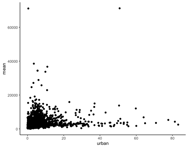
Now, I can plot the data using ggplot to look at the relationship I am interest in.
ggplot(data = mod_df, aes(x=urban, y=mean)) +
  geom_point() +
  theme_classic()
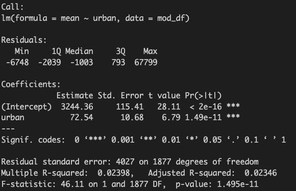
Then, I can create a linear model.
mod <- lm(mean ~ urban, data = mod_df)
summary(mod)
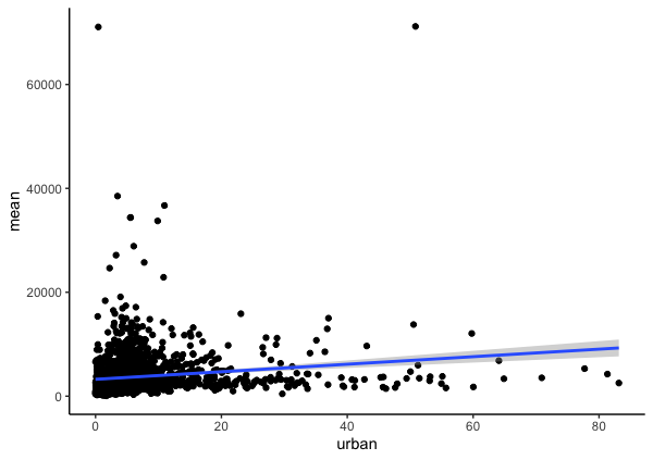
Finally, I can plot the data with the model.
ggplot(data = mod_df, aes(x=urban, y=mean)) +
  geom_point() +
  stat_smooth(method = 'lm') +
  theme_classic()
Tableau
Next, I want to demonstrate the use of the DB by connecting it to Tableau and creating an interactive dashboard. Specifically, this dashboard is intended to allow viewers to see the quantity and locations of data across the US. I plan to create an interactive map and bar graph that allows viewers to see the counts of observation in the data across space and time. In order to accomplish that type of visualization I will need access to at least 4 of the tables in the DB.
1. First, I need to open up a new tableau project.
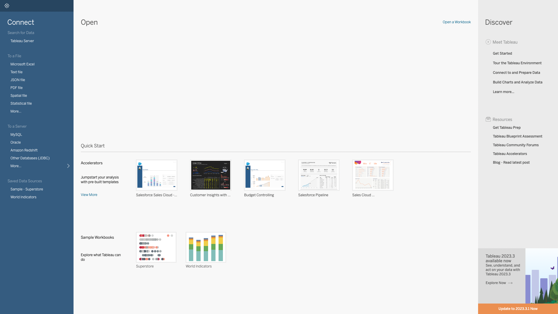
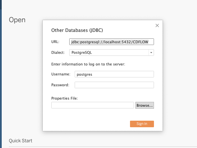
2. Connect to my local Postgres server.
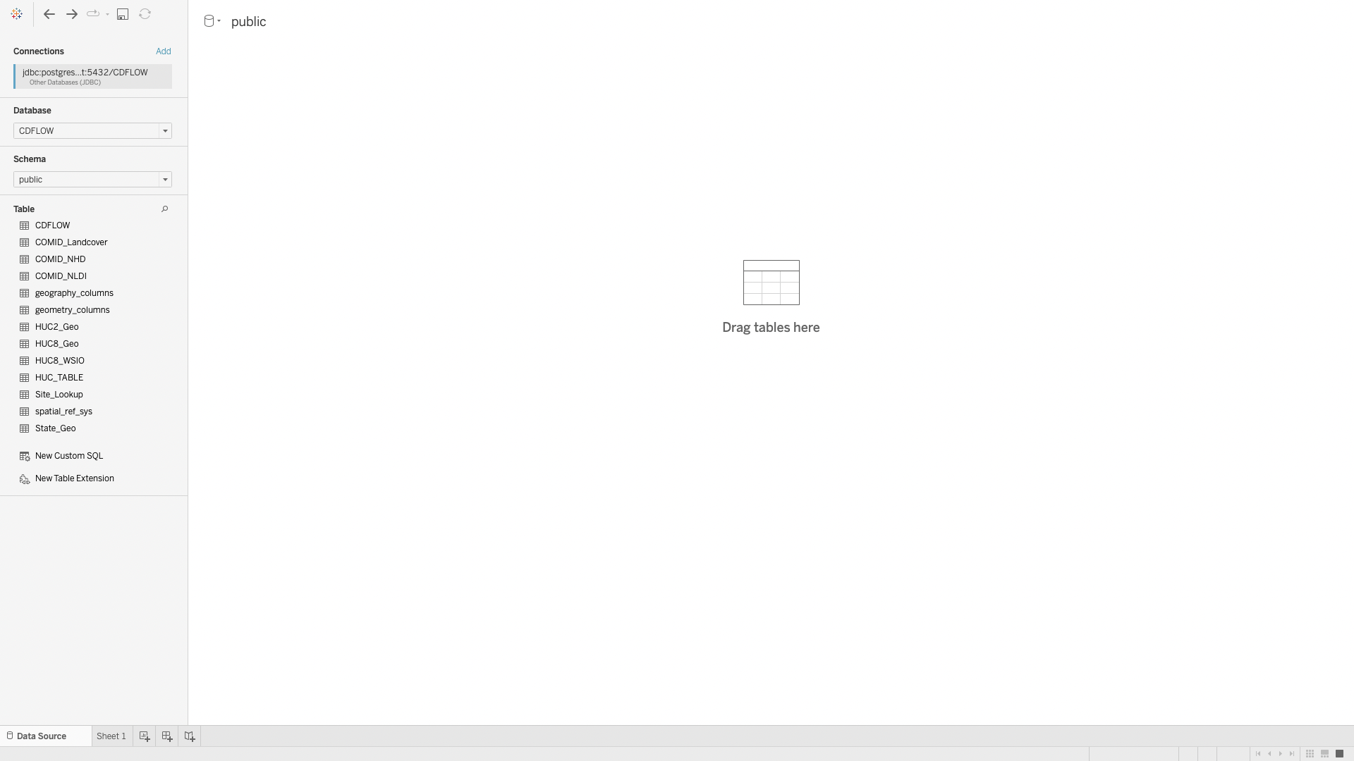
3. See the tables available.
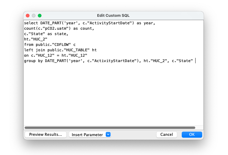
However, there is an issue. The data is too much for Tableau to handle. The good news is that Tableau allows for the use of custom SQL queries!
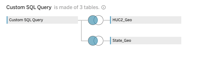
4. Create custom SQL query.
I want to get the counts of data grouped by year, state, and huc2.
5. Join with spatial tables from DB.
I can add the spatial tables straight to tableau and setup the connections with a couple of left joins.
6. Create Dashboard!
The point of this project is to demonstrate relational database skills not Tableau skills, so I’ll skip the creation of the Dashboard. However, below you can see the final product!
Note: this dashbaord is included in my tableau data visualization portfolio project.

Conclusion
From gaining insight through industry data to academic research pursuits relational databases are a powerful tool for Data Scientists. In this project I went through the creation, design, and implementation of a relation DB. Additionally, I demonstrated use cases of the DB by querying data to create a model and connecting the DB to Tableau to create an interactive data visualization.
Thanks for reading!